An Introduction to Support Vector Machines (SVM): Gradient Descent Solution

Just to clarify, these contents are mainly summarized from the course I took: “Fundamental of Big Data Analytics”, taught by Prof. Mathar Rudolf. For for information please visit: https://www.ti.rwth-aachen.de

In the last post, we discussed that the SVM optimization problem is:

$$\text{min}\frac{1}{2}\|\mathbf{w}\|^2,\ \ \text{s.t.}\ \ \ y_i(\mathbf{w}^T\mathbf{x}_i+b)\geq 1, \ \ i=1,\dots,n$$

To solve this optimization problem, there are multiple ways. One way is to treat this problem as a standard optimization problem and use gradient descent algorithm to compute the optimal parameters. Another way is to formulate the Lagrangian dual problem of the primal problem, transferring original optimization problem into an easier problem. Here we mainly discuss the first method.

Gradient Descent Algorithm

To apply GD, we need to design a new objective function which is differentiable. The new objective function is:

$$\text{min}_{\mathbf{w},b}\ L=\frac{\lambda}{2}\|\mathbf{w}\|^2+\frac{1}{n}\sum^{n}_{i=1}{\max\{1-y_i(\mathbf{w}^T\mathbf{x}_i+b) ,0\}}$$

This objective function contains two terms. The first term is used to maximize the margin. This term is also called regularization term. The second term is a penalty term used to penalize the case where \(y_i(\mathbf{w}^T\mathbf{x}_i+b)<1\), which represents incorrect/imperfect classification. Note that for the case \(y_i(\mathbf{w}^T\mathbf{x}_i+b)\geq 1\) we don’t need to penalize it, so we use a max function \(\max\{1-y_i(\mathbf{w}^T\mathbf{x}_i+b) ,0\}\). This is also called hinge loss.

$$ h(z) = \max\{1-z, 0\} $$

It looks like a hinge, isn't it?

\(\lambda\) is a weight parameter used to control the weight of the regularization term. If \(\lambda\) is too small, the model (the learned hyperplane) will mainly focuses on correctly classify the training data, but the margin may not be maximized. If \(\lambda\) is too large, the model will have have a large margin, while there may exist more miss-classified points in the training dataset.

Compute the gradient
To apply GD we also need get the exact expression of the gradient.

$$\frac{\partial{L}}{\partial{\mathbf{w}}}=\lambda\mathbf{w}-\frac{1}{n}\sum_{i=1}^{n}{u(1-y_i(\mathbf{w}^T\mathbf{x}_i+b))y_i\mathbf{x}_i} $$ $$ \frac{\partial{L}}{\partial{b}}=-\frac{1}{n}\sum_{i=1}^{n}{u(1-y_i(\mathbf{w}^T\mathbf{x}_i+b))y_i} $$

where

$$u(z)=\begin{cases} 1, & \text{if $z>0$}.\\ 0, & \text{otherwise}. \end{cases}$$

The updating rules of the parameter \(\mathbf{w}\) and \(b\) are:

$$ \mathbf{w}\leftarrow \mathbf{w} - \alpha\frac{\partial{L}}{\partial{\mathbf{w}}}\\ b\leftarrow b - \alpha\frac{\partial{L}}{\partial{b}}\\ $$

where \(\alpha\) is the learning rate.

Note that in practice that in each update loop we may not use the whole training dataset, instead we may use a mini-batch. Suppose that the mini batch size is \(m\), then the expression of the gradient is:

$$ \frac{\partial{L}}{\partial{\mathbf{w}}}=\lambda\mathbf{w}-\frac{1}{m}\sum_{i=1}^{m}{u(1-y_i(\mathbf{w}^T\mathbf{x}_i+b))y_i\mathbf{x}_i}\\ \frac{\partial{L}}{\partial{b}}=-\frac{1}{m}\sum_{i=1}^{m}{u(1-y_i(\mathbf{w}^T\mathbf{x}_i+b))y_i} $$

In the following we will use this mini-batch style expression.

Code Implementation

To test the GD algorithm, we use toy data shown in figure 2d toy data

2d toy data In this dataset, each \(\mathbf{x}_ i\) is an 2 dimensional vector. In total there are 2000 samples. We need to use GD to find the optimal separating hyperplane, which is a line in this case. The code is available in my github: SupportVectorMachine/gd-svm.py.

Experiment and Analysis

Visualization of Hyperplane
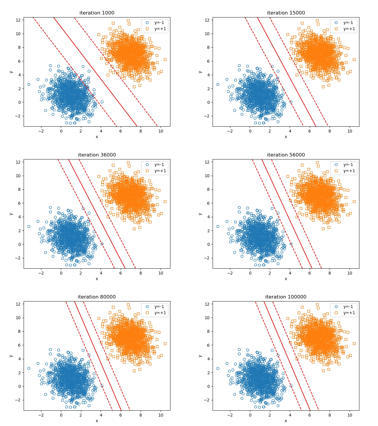
In this part, we set \(\lambda=1e-4, \text{learning_rate}=0.1, \text{batch_size}=100, \text{maximum_iteration}=100000\). The change of the hyperplane over iterations is shown in figure Hyperplane Over Iteration

Hyperplane Over Iteration After 100000 iterations the hyperplane looks accurate and the margin seems to be maximized. If we compare the final result with the SVM illustration figure, we will find that they are very similar, which implies that the gradient descent algorithm does work! Comparison between experiment results and model illustration Influence of \(\lambda\) on the final results
We can also test the influence of \(\lambda\) on the final results of the hyperplane, to check if our illustration on \(\lambda\) above is right or not. The results are shown in figure Influence Of Lambda. Influence Of Lambda The results are within our expectation. When \(\lambda\) is too large, like 0.1, the margin is very large, but there are actually some points inside the margin area, which means that the constraints \(y_i(\mathbf{w}^T\mathbf{x}_ i+b)\geq 1\) is not satisfied for some points. when \(\lambda\) is smaller, the margin becomes smaller, but all points satisfy the constraint.

We also noticed that when \(\lambda\) is extremely small, like 1e-5, the margin doesn’t become further smaller. Actually we tested that even if \(\lambda=0\) we will still get the same ideal results, which implies that the regularization term in the loss function is useless in this toy example! This may be due to the fact that for such a simple dataset, it is very easy to find the optimal separating hyperplane and support vectors. Once the optimal separating hyperplane is found, the model will stick to it even if there is no regularization term in the loss function, since in this case the gradient is 0, and the training is actually stopped.

Use SVM for classification

Suppose that we have obtained the optimal \(\mathbf{w}^{\star}\) and \(b^{\star}\), given a new input data \(\mathbf{x}\), we can make a decision of the label \(\hat{y}\) in two ways:

Hard Decision
\(\hat{y}=\begin{cases} +1, & \text{if}\ {\mathbf{w}^{\star}}^T\mathbf{x} +b^{\star}\geq 0\\ -1, & \text{if}\ {\mathbf{w}^{\star}}^T\mathbf{x} +b^{\star} < 0\\ \end{cases}\)

Soft Decision
\(\hat{y} = d( {\mathbf{w}^{\star}}^T\mathbf{x} +b^{\star} )\)
where \(d(z) = \begin{cases} 1, & \text{if}\ z \geq 1 \\ z, & \text{if}\ -1 \leq z < 1\\ -1, & \text{if}\ z < -1\\ \end{cases}\)

So that’s it. Now we are able to use GD to train a SVM model and used it for classification task. In the next post we will explore more possibilities of the solutions on SVM.

---

• Previous
  An Introduction to Support Vector Machines (SVM): Basics
• Next
  An Introduction to Support Vector Machines (SVM): Convex Optimization and Lagrangian Duality Principle

---