An Introduction to Support Vector Machines (SVM): SVM with slack variables

Just to clarify, these contents are mainly summarized from the course I took: “Fundamental of Big Data Analytics”, taught by Prof. Mathar Rudolf. For for information please visit: https://www.ti.rwth-aachen.de

Recall of the SVM primal problem:

$$ \min_{\mathbf{w},b}\ \frac{1}{2}\|\mathbf{w}\|^2\\ \begin{align} s.t.\ \ & y_i(\mathbf{w}^T\mathbf{x}_i+b)\geq 1,\ i=1,\dots,n \end{align} $$

This is the primal problem of the SVM in the case where points of two classes are linearly separable. Such a primal problem has two drawbacks:

The separating plane is sensitive to (easily influenced by) outliers.
Not suitable for the case where points of two classes are not linearly separable.

The separating plane is sensitive to (easily influenced by) outliers. Hyperplane Influenced by Outliers Figure Hyperplane Influenced by Outliers shows how a single outlier greatly influences the final results of the hyperplane. This is due to the constraints $y_i(\mathbf{w}^T\mathbf{x}_ i+b)\geq 1$ in the primal problem will make sure that the minimum geodesic distance between points and the separating hyperplane is $\frac{1}{\|\mathbf{w}\|}$. When there is an outlier, in order to satisfy the constraints, the model will choose a smaller $\|\mathbf{w}\|$ and also greatly change the rotation/position of the separating hyperplane. However, using the separating hyperplane in Figure (b) is not a good choice, since compared with (a), in (b) the points have a much smaller average geodesic distance to the separating hyperplane. Therefore, it is more likely that the SVM makes wrong decisions when classifying new points.
Not suitable for the case where points of two classes are not linearly separable.
If the points are not linearly separable, then the SVM primal problem doesn’t have a optimal solution, since there doesn’t exist a certain $\mathbf{w}$ and $b$ which satisfies the constraints $y_i(\mathbf{w}^T\mathbf{x}_ i+b)\geq 1$.

SVM with Slack Variables

To solve the problems above, we need to introduce a slack variable to the original SVM primal problem. This means that we allow certain (outlier) points to be within the margin or even cross the separating hyperplane, but such cases would be penalized. Now the primal problem of the “Slack-SVM” will be:

Primal Problem

$$ \min_{\mathbf{w},b}\ \frac{1}{2}\|\mathbf{w}\|^2 + C \sum_{i=1}^{n}\xi _i \\ \begin{align} s.t.\ \ y_i(\mathbf{w}^T\mathbf{x}_i+b) &\geq 1-\xi_i ,\ &i=1,\dots,n \\ \xi_i &\geq 0,\ &i=1,\dots,n \end{align} $$

Here $\xi_i$ is the slack variable, and the positive $C$ is the weight for the penalty term. Suppose that for some point $\mathbf{x}_i$, it holds $y_i(\mathbf{w}^T\mathbf{x}_i+b) = 1-\xi_i$:

if $\xi_i=0$, then $\mathbf{x}_i$ is exactly at the marginal hyperplane (the margin for short).
if $0<\xi_i\leq 1$, then $\mathbf{x}_i$ is located within the margin, but the label of $\mathbf{x}_i$ is correctly classified.
if $\xi_i > 1$, then $\mathbf{x}_i$ is located at the other side of the separating hyperplane, which means a miss-classification. Different $\xi$ and Point Locations

It is possible to use Gradient Descent algorithm to solve the primal problem. However, due to the slack variables, the constraints is much more complex than the case without slack variables. It is more difficult to define the loss function used for gradient descent. On the contrary, the Lagrangian dual problem of this primal problem still remains compact and solvable, and can be easily extended to kernel SVM. Therefore, in the next, we mainly discuss the deduction of the Lagrangian dual problem of the Slack SVM primal problem.

Lagrangian Function

$$L( \mathbf{w}, b, \mathbf{\xi}, \lambda, \mu )= \frac{1}{2}\|\mathbf{w}\|^2 + C\sum_{i=1}^{n}\xi_i + \sum_{i=1}^{n}\lambda_i ( 1-\xi_i - y_i(\mathbf{w}^T\mathbf{x}_ i+b ) ) - \sum_{i=1}^{n}\mu_i \xi_i $$

Lagrangian Dual function

$$ g(\lambda, \mu) = \inf_{\mathbf{w}, b, \xi} L(\mathbf{w}, b, \xi, \lambda, \mu) $$

To get the dual function, we can compute the derivative and set them to 0.

$$ \frac{\partial{L}}{\partial{\mathbf{w}}} = \mathbf{w} - \sum_{i=1}^{n}\lambda_i y_i \mathbf{x}_i = 0 \\ \frac{\partial{L}}{\partial{b}} = -\sum_{i=1}^{n}\lambda_i y_i = 0\\ \frac{\partial{L}}{\partial{\xi_i}} = C - \lambda_i - \mu_i = 0 $$

From these 3 equations we have

$$ \mathbf{w}^\star = \sum_{i=1}^{n} \lambda_i y_i \mathbf{x}_i\\ \sum_{i=1}^{n} \lambda_i y_i = 0\\ \mu_i = C-\lambda_i $$

Substitue them in the Lagrangian function, we can get the Lagrangian dual function:

$$ g(\lambda, \mu) = \frac{1}{2}\sum_{i,j}\lambda_i \lambda_j y_i y_j \mathbf{x}_i^T\mathbf{x}_j + C\sum_{i=1}^{n}\xi_i + \sum_{i=1}^{n}\lambda_i -\sum_{i=1}^{n}\lambda_i \xi_i \\-\sum_{i,j}\lambda_i \lambda_j y_i y_j \mathbf{x}_i^T\mathbf{x}_j - \sum_{i=1}^{n}\lambda_i y_i b - C\sum_{i=1}^{n}\xi_i + \sum_{i=1}^{n}\lambda_i \xi_i\\ = \sum_{i=1}^{n}\lambda_i - \frac{1}{2}\sum_{i,j}\lambda_i \lambda_j y_i y_j \mathbf{x}_i^T\mathbf{x}_j $$

Therefore, the Lagrangian dual problem is:

$$ \max_{\lambda, \mu} \sum_{i=1}^{n}\lambda_i - \frac{1}{2}\sum_{i,j}\lambda_i \lambda_j y_i y_j \mathbf{x}_i^T\mathbf{x}_j\\ \begin{align} s.t.\ & \lambda_i \geq 0\\ &\mu_i \geq 0 \\ &\mu_i = C-\lambda_i \\ &\sum_{i=1}^{n} \lambda_i y_i =0 \end{align} $$

We can use $\lambda_i$ to represent $\mu_i$, and finally get the dual problem:

Dual Problem

$$ \max_{\lambda, \mu} \sum_{i=1}^{n}\lambda_i - \frac{1}{2}\sum_{i,j}\lambda_i \lambda_j y_i y_j \mathbf{x}_i^T\mathbf{x}_j\\ \begin{align} s.t.\ & 0 \leq \lambda_i \leq C \\ &\sum_{i=1}^{n} \lambda_i y_i =0 \end{align} $$

Compared with the dual problem for the SVM without slack variables, the only difference is that here the constraints of $\lambda$ are $0\leq \lambda_i \leq C$, instead of $\lambda_i \geq 0$.

Actually in the primal problem of the SVM without slack variables, we can think there is a hidden $C=\infty$, which means that the penalty of slack variables is infinitely large, so all points need to satisfy $y_i(\mathbf{w}^T\mathbf{x}_ i+b)\geq 1$.

Solution of the Dual Problem

Gradient Descent Algorithm The objective function for gradient descent is:
$$ \min_{\lambda} L(\lambda) = -\sum_{i=1}^{n} \lambda_i + \frac{1}{2}\sum_{i,j}\lambda_i \lambda_j y_i y_j \mathbf{x}_ i^T \mathbf{x}_ j + \frac{c}{2}(\sum_{i=1}^{n}\lambda_i y_i)^2 \\ s.t.\ 0\leq \lambda_i \leq C \ , \ i=1,\dots,n $$ Compared with the post An Introduction to Support Vector Machines (SVM): Dual problem solution using GD, the objective function is the same. The only difference is that here the constraints are $0\leq \lambda_i \leq C$. To achieve this constraints, we can clip the value of $\lambda_i$ in the range $[0,C]$ after each gradient descent back propagation. For the detail of the gradient form, please have a look at that post.
Sequential Minimal Optimization (SMO), which will be discussed in the following posts.

Discussion on the Karush-Kuhn-Tucker (KKT) conditions The KKT conditions are now slightly different, since now in the dual function there are actually two variables: $\lambda$ and $\mu$. For the primal optimum $\mathbf{w}^\star, b^\star, \xi^\star$ and the dual optimum $\lambda^\star, \mu^\star$, it holds:

primal constraints $$ y_i({\mathbf{w}^\star}^T\mathbf{x}_ i +b^\star) \geq 1-\xi^\star_i \\ \xi^\star_i \geq 0 $$
compute the infimum of $L$ w.r.t $\mathbf{w}$ and $\xi$ $$ \Delta_{\mathbf{w},b,\xi}L( \mathbf{w}^\star, b^\star, \xi^\star, \lambda^\star, \mu^\star)=0 $$
dual constraints $$ \lambda_i^\star \geq 0\\ \mu_i^\star \geq 0\\ \sum_{i=1}^{n}\lambda_i^\star y_i =0\\ \mu_i^\star = C - \lambda_i^\star $$
Complementary Slackness $$ \lambda_i^\star ( 1-\xi_i^\star - y_i({\mathbf{w}^\star}^T\mathbf{x}_ i +b^\star ) ) =0 \\ \mu_i^\star \xi_i^\star = 0 $$

The complementary slackness is interesting. Suppose that we have already find the primal optimum and dual optimum. We can analyze the location of the point $\mathbf{x}_ i$ based on the value of $\lambda_i$:

$\lambda_i^\star=0$
then $\mu_i^\star = C$, so $\xi^\star_i=0$, and $y_i({\mathbf{w}^\star}^T\mathbf{x}_ i+b^\star)\geq 1$. This means the distance from point $\mathbf{x}_ i$ to the separating hyperplane is greater than or equal to $\frac{1}{\|\mathbf{w}^\star\|}$. This point $\mathbf{x}_ i$ is not support vector.
$0<\lambda_i^\star<C$
then $0<\mu_i^\star<C$, so $\xi_i^\star =0$, and $y_i({\mathbf{w}^\star}^T\mathbf{x}_ i+b^\star)=1$. This means that $\mathbf{x}_ i$ is exactly located at the margin hyperplane: the distance to the separating hyperplane is exactly $\frac{1}{\|\mathbf{w}^\star\|}$. The point $\mathbf{x}_ i$ is a support vector which is used to compute $\mathbf{w}^\star$ and $b^\star$.
$\lambda_i^\star = C$
then $\mu_i^\star =0$, so $\xi^\star_i\geq 0$, and $y_i({\mathbf{w}^\star}^T\mathbf{x}_ i+b^\star)=1-\xi^\star_i$. This means that $\mathbf{x}_ i$ is within the margin, or even located in the other side of the separating hyperplane (miss-classification). The point $\mathbf{x}_ i$ is also a support vector which is used to compute $\mathbf{w}^\star$, but not used to compute $b^\star$.

Suppose that we have solved the dual problem and get the dual optimum. Let $S_w=\{ i \vert 0<\lambda_i^\star \leq C \}$ represent the support set related with $\mathbf{w}$; $S_b=\{ i \vert 0<\lambda_i^\star < C \}$ represent the support set related with $b$. Meanwhile, we define $S_b^+ =\{ i \vert i\in S_b \ \text{and}\ y_i = +1 \}$ and $S_b^-=\{ i \vert i\in S_b\ \text{and}\ y_i = -1 \}$. Then we can compute the primal optimum:

$$ \mathbf{w}^\star = \sum_{i\in S_w}\lambda_i^\star y_i \mathbf{x}_i $$

Multiple ways can be used to compute $b^\star$:

$$ b^\star= y_i - {\mathbf{w}^\star}^T\mathbf{x}_i \ , \ i\in S_b\\ b^\star= \frac{1}{\vert S_b \vert}\sum_{i\in S_b}({y_i - {\mathbf{w}^\star}^T\mathbf{x}_i})\\ b^\star = -\frac{1}{2}{\mathbf{w}^\star}^T(\mathbf{x}_i+\mathbf{x}_j)\ , \ i\in S_b^+, j \in S_b^- $$

Experiment Results

We compare the separating hyperplane results between the SVM with slack variables (Slack-SVM for short) and the original SVM without slack variables (Original-SVM for short). The SVM models are trained by solving the Lagrangian dual problem using gradient descent algorithm introduced in the last post.

For further discussion, we recall the primal/dual problem of the Original-SVM and the primal/dual problem of the Slack-SVM:

Original-SVM
Primal Problem $$ \min_{\mathbf{w},b}\ \frac{1}{2}\|\mathbf{w}\|^2\\ \begin{align} s.t.\ \ & y_i(\mathbf{w}^T\mathbf{x}_ i+b)\geq 1,\ i=1,\dots,n \end{align} $$ Dual Problem $$ \max_{\lambda, \mu} \sum_{i=1}^{n}\lambda_i - \frac{1}{2}\sum_{i,j}\lambda_i \lambda_j y_i y_j \mathbf{x}_i^T\mathbf{x}_j\\ \begin{align} s.t.\ & \lambda_i \geq 0 \\ &\sum_{i=1}^{n} \lambda_i y_i =0 \end{align} $$
Slack-SVM
Primal Problem $$ \min_{\mathbf{w},b}\ \frac{1}{2}\|\mathbf{w}\|^2 + C \sum_{i=1}^{n}\xi _i \\ \begin{align} s.t.\ \ y_i(\mathbf{w}^T\mathbf{x}_ i+b) &\geq 1-\xi_i ,\ &i=1,\dots,n \\ \xi_i &\geq 0,\ &i=1,\dots,n \end{align} $$ Dual Problem $$ \max_{\lambda, \mu} \sum_{i=1}^{n}\lambda_i - \frac{1}{2}\sum_{i,j}\lambda_i \lambda_j y_i y_j \mathbf{x}_i^T\mathbf{x}_j\\ \begin{align} s.t.\ & 0 \leq \lambda_i \leq C \\ &\sum_{i=1}^{n} \lambda_i y_i =0 \end{align} $$

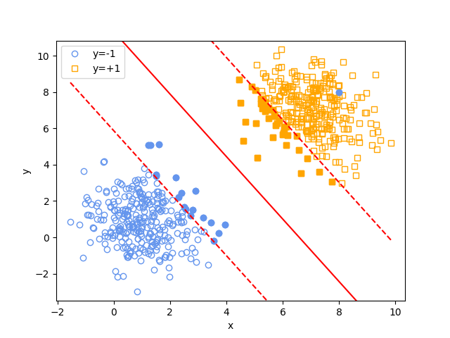
Experiment 1.
Comparison of performance in the case where there are outliers but the points are still linearly separable. The Slack-SVM penalty term weight $C=0.5$

Slack SVM vs Original SVM on separable outliers This result fits well with the analysis in the Figure Hyperplane Influenced by Outliers! The original SVM tries hard to find a separating hyperplane regardless of the obvious outlier point. It takes $2\times 10^6$ iterations (20 times longer than Slack SVM) to finally find the separating hyperplane with a tight margin. On the contrary, the Slack SVM simply chooses to ignore the outlier point. The separating hyperplane is almost identical to the case without the outlier point.

Experiment 2.
Analyzing the influence of different Slack-SVM penalty term weight $C$.

Slack SVM over different penalty weight C

As we increase the value of $C$, the geodesic margin becomes wider. The outlier point is closer to the margin hyperplane geodesically. More points become support vectors.

To explain this we need to refer the form of the Slack SVM primal problem. When we increase $C$, the penalty term $C\sum_{i=1}^{n}\xi_i$ is more heavily penalized. The model tends to reduce the value of $\xi_i$. So how to reduce $\xi_i$ ?

The answer is to reduce $\|\mathbf{w}\|$. This may sound a little bit bizarre, but we can tell that from the figure Slack SVM over different penalty weight C.

For different value of $C$, the location and rotation of the separating hyperplane remains similar, so the distance from points to the separating hyperplane is similar. We know that for a point $\mathbf{x}_ i$ which is within the margin or is located in the other side of the separating hyperplane, its geodesic distance to the separating hyperplane is $\frac{\vert 1-\xi_i \vert}{\|\mathbf{w}\|}$. For the outlier points which cross the separating hyperplane, like the solid blue circle in the top right corner, the geodesic distance is $\frac{\xi_i -1 }{\|\mathbf{w}\|}$.

Since for large $C$, we need to reduce the large $\xi_i$ of that outlier point, with the fact that the geodesic distance remains unchanged. So the possible solution is to reduce $\|\mathbf{w}\|$. As a result, the geodesic margin $\frac{1}{\|\mathbf{w}\|}$ will be increased. Therefore, the larger $C$ is, the wider the margin area is.

Original SVM for linearly non-separable cases
We also notice that for $C=100$ and $C=10000$, the separating results are almost the same. This leads to another question: what if we set $C=\infty$ and solve the dual problem of the Slack SVM?

If we set $C=\infty$, the primal/dual problem of the Slack SVM is exactly the same as the primal/dual problem of the original SVM. This is the short proof:

for dual problem, it obviously holds.
for primal problem: $$ \min_{\mathbf{w},b}\ \frac{1}{2}\|\mathbf{w}\|^2 + C \sum_{i=1}^{n}\xi _i \\ \begin{align} s.t.\ \ y_i(\mathbf{w}^T\mathbf{x}_ i+b) &\geq 1-\xi_i ,\ &i=1,\dots,n \\ \xi_i &\geq 0,\ &i=1,\dots,n \end{align} $$ When $C\rightarrow \infty$, to minimize the objective function into some finite value, it must hold $\xi_i \equiv 0$. Therefore, $C \sum_{i=1}^{n}\xi _ i=0$, and the Slack SVM’s primal problem will be: $$ \min_{\mathbf{w},b}\ \frac{1}{2}\|\mathbf{w}\|^2 \\ \begin{align} s.t.\ \ y_i(\mathbf{w}^T\mathbf{x}_ i+b) &\geq 1,\ &i=1,\dots,n \\ \end{align} $$ This is exactly the Original SVM’s primal problem.

Therefore, the above question is equivalent to ask: What if we apply the Original SVM to the linearly non-separable case?

The answer is that the separating results will be almost the same as the case $C=10000$ in the figure Slack SVM over different penalty weight C. Why the geodesic margin is not further enlarged?

We showed that original SVM is equivalent to set $C=\infty$ in Slack-SVM. However, from the aspect of the dual problem, the real value of $C$ is actually determined by the up-bound of $\lambda$. For example, if we set $C=\infty$, but the real up-bound of the trained $\lambda$ is 10000, then the real effective $C$ is actually 10000. Therefore, we will see by applying Original SVM to linearly non-separable case, the final separating result is identical to the $C=10000$ case.

Original SVM on linearly non-separable case Here I also check the maximum of $\lambda$ after the training for different $C$

$C$	10	100	10000	$\infty$
$\max{\lambda}$	10	62.2	62.2	62.2

We can see that when $C$ reaches 100, the maximum of $\lambda$ usually reaches around 60. Therefore, keeping increasing $C$ does not influence the separating results further. Note that as we continue training, the $\max{\lambda}$ may further rise, but it can hardly reach the value of $C$ if $C$ is very large.

An Introduction to Support Vector Machines (SVM): SVM with slack variables

支持向量机(SVM)概述：具有松弛变量的支持向量机

SVM with Slack Variables

Experiment Results

CATALOG

FEATURED TAGS

FRIENDS