An Introduction to Expectation-Maximization (EM) Algorithm

Expectation Maximization (EM) algorithm is a special case of MLE where the observations (data samples $\mathbf{x}$) are inherently related with some hidden variables ($\mathbf{z}$). First of all, we need to review the basics of MLE.

Maximum Likelihood Estimation (MLE)

Let $\{\mathbf{x}^{(i)}\},\ i=1,\dots,n$ be a set of independent and identically distributed observations, and $\mathbf{\theta}$ be the parameters of the data distribution which are unknown for us. The maximum likelihood estimation of the parameters $\theta$ is the parameters which can maximize the joint distribution $p_\theta(\mathbf{x}^{(1)},\dots,\mathbf{x}^{(n)})= \prod_{i=1}^{n}p_\theta(\mathbf{x}^{(i)})$

$$ \hat{\theta}_\text{MLE} = \arg\ \max_{\theta}{\prod_{i=1}^{n}p_\theta(\mathbf{x}^{(i)})} $$

More commonly, we choose to maximize the joint log-likelihood:

$$ \hat{\theta}_\text{MLE} = \arg\ \max_{\theta}{\sum_{i=1}^{n}\log p_\theta(\mathbf{x}^{(i)})} $$

We use an example to illustrate how it works (referred from EM算法详解-知乎).

Suppose that we have a coin A, the likelihood of a heads is $\theta_A$. We denote one observation $\mathbf{x}^{(i)}=\{ x_ {i,1},x_ {i,2},x_ {i,3},x_ {i,4},x_ {i,5}, \}$ as tossing the coin A 5 times and record the heads (1) or tails (0) of each tossing. For example, $\mathbf{x}^{(i)}$ can be 01001, 01110, 10010, … etc. The likelihood of the observation $\mathbf{x}^{(i)}$ is:

$$ p({\mathbf{x}^{(i)}}) = \prod_{j=1}^{5}\theta_A^{x_{i,j}}(1-\theta_A)^{1-x_{i,j}} = \theta_A^{\sum_{j=1}^{5}x_{i,j}}(1-\theta_A)^{\sum_{j=1}^{5}(1-x_{i,j})} $$

Therefore, the log likelihood of the joint distribution of $n$ observations is:

$$ l(\theta_A) = \sum_{i=1}^{n} \sum_{j=1}^{5}\Big( x_{i,j}\log{\theta_A} +(1-x_{i,j})\log{(1-\theta_A)} \Big) $$

The MLE of $\theta_A$ is

$$ \hat{\theta}_{A,\text{MLE}} = \arg \max_{\theta_A} l(\theta_A) $$

To get $\hat{\theta}_{A,\text{MLE}}$ we can solve the equation $\frac{\partial{l(\theta_A)}}{\partial{\theta_A}}=0$.

$$ \begin{align} \frac{\partial{l(\theta_A)}}{\partial{\theta_A}} &= \sum_{i=1}^{n}\sum_{j=1}^5 \Big(\frac{x_{i,j}}{\theta_A} + \frac{x_{i,j}-1}{1-\theta_A} \Big)\\ &= \frac{\sum_{i=1}^{n}\sum_{j=1}^5 x_{i,j}}{\theta_A} + \frac{\sum_{i=1}^{n}\sum_{j=1}^5 x_{i,j}-5n}{1-\theta_A} \\ &= 0 \end{align} $$

Therefore, we have

$$ \hat{\theta}_{A, \text{MLE}} = \frac{\sum_{i=1}^{n}\sum_{j=1}^5 x_{i,j}}{5n} $$

This is actually equivalent to compute the average value of all tossing results. For example, if we have 10 observations as below:

$\mathbf{x}^{(1)}$	01011	$\mathbf{x}^{(6)}$	01110
$\mathbf{x}^{(2)}$	01111	$\mathbf{x}^{(7)}$	01110
$\mathbf{x}^{(3)}$	11011	$\mathbf{x}^{(8)}$	11011
$\mathbf{x}^{(4)}$	00011	$\mathbf{x}^{(9)}$	00100
$\mathbf{x}^{(5)}$	01010	$\mathbf{x}^{(10)}$	01001

The sum of all tossing is 28, and the total number of tossing is 50, so MLE of $\theta_A$ is $\frac{28}{50}=\frac{14}{25}$

MLE with hidden variables

Now things become more complicated. Suppose we have two coins: A and B. The likelihood of a heads of coin A and B are $\theta_A$ and $\theta_B$ respectively. We want to find the MLE of $\theta_A, \theta_B$ using $n$ observations $\{\mathbf{x}^{(i)}\},\ i=1,\dots,n$. Each observation has the same form as above. The challenging part is that for each observation $\mathbf{x}^{(i)}$, we don’t know which coin it comes from. For example, $n=10$, the observation set is the same as the table above. In this case how to find the MLE of $\theta_A$ and $\theta_B$?

This is an simple example where our observation is closely related with some hidden (unknown) variables. In other words, the information of the data is incomplete. The Expectation-Maximization algorithm can be used to solve these problems.

Expectation-Maximization (EM) Algorithm

Before introducing EM algorithm, we need to known an important inequality: Jensen-Shannon Inequality.

Jensen-Shannon Inequality

If a function $f(\mathbf{X})$ is strictly convex, where $\mathbf{X}$ is a random variable and the Hessian matrix $H$ is positive definite, we have

$$ E_{X}[f(\mathbf{X})] \geq f(E_X(\mathbf{X})) $$

The equality holds if and only if $E_X [\mathbf{X}]= \mathbf{X}$ with the probability 1 ($\mathbf{X}$ is a constant). Note that of $f(\mathbf{X})$ is strictly concave, the direction of the inequality needs to be reversed.

We can use an example to illustrate Jensen-Shannon inequality more intuitively (not proof). This example is referred from Andrew Ng’s lecture note on EM. As shown in this figure, the random variable $\mathbf{X}$ has only two possible values: $a$ and $b$, each with the probability 0.5. Therefore, $f(E[\mathbf{X}])= f(\frac{a+b}{2})$ and $E[f(\mathbf{X})]=\frac{f(a)+f(b)}{2}$. According to the convexity of the function $f(\mathbf{X})$, we have $E[f(\mathbf{X})]\geq f(E[\mathbf{X}])$, and the equality holds if and only if $a=b$, which means $E[\mathbf{X}]=\mathbf{X}=a$.

Now we have a powerful tool, and we will use it to deduce the EM algorithm.

EM algorithm
Recall the MLE problem:

$$ \theta_\text{MLE} = \arg \max_{\theta} \sum_{i=1}^{n} \log{p_\theta(\mathbf{x}^{(i)})} $$

If $\mathbf{x}$ is related with a latent variable $\mathbf{z}$, we write $p_\theta$ as the marginal likelihood of the joint distribution:

$$ p_\theta(\mathbf{x}^{(i)}) = \sum_{z} p_\theta(\mathbf{x}^{(i)}, \mathbf{z}) $$

Now our log-likelihood function $l(\theta)$ becomes:

$$ l(\theta) = \sum_{i=1}^{n}\log \sum_{z} p_\theta(\mathbf{x}^{(i)}, \mathbf{z}) $$

The expression of the joint distribution is not known to us. To solve this maximization problem we introduce a distribution $Q^{(i)}(\mathbf{z})$, and rewrite the log-likelihood function as:

$$ \begin{align} l(\theta) &= \sum_{i=1}^{n} \log \sum_{z} Q^{(i)}(z) \frac{p_\theta(\mathbf{x}^{(i)},\mathbf{z}))}{Q^{(i)}(\mathbf{z})}\\ &= \sum_{i=1}^{n} \log E_{z\in Q^{(i)}(z)} \left[ \frac{p_\theta(\mathbf{x}^{(i)},\mathbf{z}))}{Q^{(i)}(\mathbf{z})}\right] \end{align} $$

We know that the function $f(x)=\log(x)$ is strictly concave, so according to the Jensen-Shannon inequality, we have the following inequality:

$$ l(\theta) \geq L(\theta, Q^{(i)}) =\sum_{i=1}^{n} E_{z \in Q^{(i)}(z)}\left[ \log{\frac{p_\theta(\mathbf{x}^{(i)},\mathbf{z}))} {Q^{(i)}(\mathbf{z})}} \right] $$

The equality holds if and only if $\frac{p_\theta(\mathbf{x}^{(i)},\mathbf{z}))} {Q^{(i)}(\mathbf{z})}$ is a constant (with respect to variable $\mathbf{z}$). To achieve this we can set $Q^{(i)}(\mathbf{z})= \frac{p_\theta(\mathbf{x}^{(i)},\mathbf{z})}{\sum_{z}p_\theta(\mathbf{x}^{(i)},\mathbf{z})}= \frac{ p_\theta(\mathbf{x}^{(i)},\mathbf{z}) }{p_\theta(\mathbf{x}^{(i)})}= p_\theta(\mathbf{z}\vert \mathbf{x}^{(i)})$. This means $Q^{(i)}(\mathbf{z})$ is the posterior of $\mathbf{z}$ given $\mathbf{x}^{(i)}$.

People may ask: why do we try to find a proper $Q^{(i)}(\mathbf{z})$ to make the equality hold?

Our initial goal is to find the MLE of $\theta$ w.r.t $l(\theta)$. However, the original expression of $l(\theta)$ is not explicit, so we take advantage of the Jensen-Shannon inequality, by selecting a proper distribution of $Q^{(i)}(\mathbf{z})$, to make $l(\theta)=L(\theta, Q^{(i)})$. Then we can instead maximize $L(\theta, Q^{(i)})$ w.r.t $\theta$ to find the MLE in an iterative way.

Now, we can summarize the EM algorithm:

Heuristically (or randomly) initialize parameters $\theta$
Repeat:
- Expectation (E) step:
  Based on current parameter $\theta$ and $\mathbf{x}^{(i)}$, set $Q^{(i)}(\mathbf{z})=p_\theta(\mathbf{z}\vert \mathbf{x}^{(i)})$.
- Maximization (M) step:
  Update $\theta \leftarrow \arg \max_{\theta} \sum_{i=1}^{n}\sum_z Q^{(i)}(\mathbf{z}) \log \frac{p_\theta(\mathbf{x}^{(i)}, \mathbf{z})}{Q^{(i)}(\mathbf{z})}$

$\ \ \ \ \ \ \ \$Until: $\theta$ converges

In Andrew Ng’s lecture notes, it is proven that can guarantee that $l(\theta)$ is steadily maximized. Suppose that after $l-1$ iterations we have the log-likelihood $l(\theta_{l-1})$. At the $l^\text{th}$ iteration, after the E step, we have $L(\theta_{l-1}, Q^{(i)}_l)= l(\theta_{l-1})$; After the M step, updated $\theta_{l}$ is selected such that $L(\theta_l, Q^{(i)}_l)\geq L(\theta_{l-1}, Q^{(i)}_l)$. Then at the $l+1$ iteration, by selecting $Q^{(i)}_{l+1}$ as the posterior of $\mathbf{z}$, we have $l(\theta_l)=L(\theta_l, Q^{(i)}_{l+1})$. Therefore, we have

$$ l(\theta_l) = L(\theta_l, Q^{(i)}_{l+1}) \geq L(\theta_l, Q^{(i)}_{l}) \geq L(\theta_{l-1}, Q^{(i)}_{l}) = l(\theta_{l-1}) $$

So we have $l(\theta_{l})\geq l(\theta_{l-1})$. This guarantees that the overall log-likelihood can only keep increasing or stay unchanged, but not decrease.

This deduction shows that the EM algorithm is heading to the right direction. However, this direction may not be the ideal one. It is pretty obvious that if $l(\theta)$ is globally concave, EM algorithm can always converge at the global optimum. If $l(\theta)$ is not globally concave, the property $l(\theta_l)\geq l(\theta_{l-1})$ will guarantee that EM algorithm will converge at some point (assume that $l(\theta)$ is not delta function), but the converge point may not be globally optimum.

Moreover, the EM algorithm is sensitive to the initialization. Different initialization may results in pretty different converge points, as shown in the figure below. EM initialization As shown in this figure, if the initialization is at point $A$, then EM will converge at point $C_A$, while the EM will converge at point $C_B$ if initialization is $B$. Obviously $C_B$ is the global optimum and $C_A$ not.

So how to make EM algorithm less sensitive to initialization and be more likely to find the global optimum? One simple, straight-forward but effective way is to randomly initialize the parameters and rum EM algorithm multiple times, and choose the parameters with the largest converged log-likelihood (objective function).

Apply EM algorithm to practical questions

Tossing two coins with different heads probability

Let recall the question raised in the first section:

Suppose we have two coins: A and B. The likelihood of a heads of coin A and B are $\theta_A$ and $\theta_B$ respectively. We want to find the MLE of $\theta_A, \theta_B$ using $n$ observations $\{\mathbf{x}^{(i)}\in \{0,1\}^d\},\ i=1,\dots,n$. Each observation has $d$ dimension, which means $d$ times of tossing for each observation. The challenging part is that for each observation $\mathbf{x}^{(i)}$, we don’t know which coin it comes from. In this case how to find the MLE of $\theta_A$ and $\theta_B$?

In this case, $\mathbf{x}$ is related with a hidden variable $z$. $z$ can only have 2 values: $z=A$ for coin $A$ and $z=B$ for coin $B$. We want to apply EM algorithm to this case.

Randomly initialize $\theta_{A,0}$, $\theta_{B,0}$, and the prior distribution of $z$ is $P(z=A)$ , $P(z=B)$.

Note that the choice of prior distribution of $z$ will influence the final learned parameters very much. If the chosen prior is pretty different from the real prior, the estimated parameters will be inaccurate. To solve this problem, we can update the prior by setting the prior of current iteration as the posterior of previous iteration, averaged over all observations. This is commonly used when data comes as a sequence.
Repeat:
at the $l^\text{th}$ iteration:
- E step:
  We need to compute the posterior:$$Q^{(i)}_l(z) = P(z|\mathbf{x}^{(i)}; \theta_{l-1}) = \frac{P(\mathbf{x}^{(i)}\vert z; \theta_{l-1}) P(z) }{ P(\mathbf{x}^{(i)}) }$$ Here $\theta_{l-1}$ represents the parameter set $\{\theta_{A,l-1}, \theta_{B, l-1}\}$. Furthermore, we known that $P(z=A|\mathbf{x}^{(i)}; \theta_{l-1})+P(z=A|\mathbf{x}^{(i)}; \theta_{l-1})=1$. Moreover we have the prior $P(z=A)=0.5$ and $P(z=B)=0.5$. Therefore, we have$$\begin{align} & Q^{(i)}_{A,l}= Q^{(i)}_ l(z=A)\\=&\frac{P(\mathbf{x}^{(i)}\vert z=A; \theta_{l-1})P(z=A) }{ P(\mathbf{x}^{(i)}\vert z=A; \theta_{l-1})P(z=A) +P(\mathbf{x}^{(i)}\vert z=B; \theta_{l-1}) P(z=B) }\\ =&\frac{P(\mathbf{x}^{(i)}\vert z=A; \theta_{l-1})}{ P(\mathbf{x}^{(i)}\vert z=A; \theta_{l-1}) +P(\mathbf{x}^{(i)}\vert z=B; \theta_{l-1}) } \end{align}$$ and $$\begin{align} &Q^{(i)}_{B,l}=Q^{(i)}_ l(z=B)\\=&\frac{P(\mathbf{x}^{(i)}\vert z=B; \theta_{l-1}) }{ P(\mathbf{x}^{(i)}\vert z=A; \theta_{l-1}) +P(\mathbf{x}^{(i)}\vert z=B; \theta_{l-1}) }\end{align}$$
- M step:
  The objective function is $$\begin{align}&L(\theta_{l-1}, Q^{(i)}_l)\\ =& \sum_{i=1}^{n} \sum_z Q^{(i)}_l(z) \log \frac{P(\mathbf{x}^{(i)},z;\theta_{l-1})}{Q^{(i)}_ l(z)}\\ =& \sum_{i=1}^{n}\Big( Q_l^{(i)}(z=A)\log \frac{ P(\mathbf{x}^{(i)}|z=A; \theta_{l-1} )P(z=A) }{Q_l^{(i)}(z=A) } +\\ &\ \ \ Q_l^{(i)}(z=B)\log \frac{ P(\mathbf{x}^{(i)}|z=B; \theta_{l-1} )P(z=B) }{Q_l^{(i)}(z=B) }\Big)\\ =& \sum_{i=1}^{n} \sum_{j=1}^{d}\Big[Q_{A,l}^{(i)}\Big(x_{i,j}\log \theta_{A,l-1} +(1-x_{i,j})\log (1-\theta_{A,l-1}) \Big)+\\ &\ \ \ Q_{B,l}^{(i)}\Big(x_{i,j}\log \theta_{B,l-1} +(1-x_{i,j})\log (1-\theta_{B,l-1}) \Big)\Big]+C \end{align}$$ Where $C$ is a term which is not related with $\theta_A$ or $\theta_B$. To update $\theta$, we need to compute the partial derivate ad set them to 0: $$\begin{align} \frac{\partial{L(\theta_{l-1}, Q_l^{(i)})}}{\partial{ \theta_{A,l-1} }}= \frac{\sum_{i=1}^{n}\sum_{j=1}^{d}Q_{A,l}^{(i)}x_{i,j}}{\theta_{A,l-1}} + \frac{\sum_{i=1}^{n}\sum_{j=1}^{d}Q_{A,l}^{(i)}(x_{i,j}-1)}{1-\theta_{A,l-1}} =0 \\ \frac{\partial{L(\theta_{l-1}, Q_l^{(i)})}}{\partial{ \theta_{B,l-1} }}= \frac{\sum_{i=1}^{n}\sum_{j=1}^{d}Q_{B,l}^{(i)}x_{i,j}}{\theta_{B,l-1}} + \frac{\sum_{i=1}^{n}\sum_{j=1}^{d}Q_{B,l}^{(i)}(x_{i,j}-1)}{1-\theta_{B,l-1}} =0 \end{align}$$ By solving these two equations, we get the update rule: $$ \theta_{A,l} = \frac{ \sum_{i}^{n} \sum_{j=1}^d Q_{A,l}^{(i)} x_{i,j} }{ \sum_{i}^{n}Q_{A,l}^{(i)}d}\\ \theta_{B,l} = \frac{ \sum_{i}^{n} \sum_{j=1}^d Q_{B,l}^{(i)} x_{i,j} }{ \sum_{i}^{n}Q_{B,l}^{(i)}d} $$
- Update prior $P(z)$: $P(z=A)=\frac{1}{n}Q_{A,l}^{(i)}$, $P(z=B)=\frac{1}{n}Q_{B,l}^{(i)}$

$\ \ \ \ \ \ \ \$Until $\theta_A,\theta_B$ converges.

Implementation and Analysis

To test the effectiveness of the EM algorithm, I wrote a small demo for the coin tossing problem:

import numpy as np

## Define a tossing function, to generate our observations
## theta is the head likelihood; num is the number of tossing for a single observation
def tossing( theta, num ):
	return (np.random.uniform(size=num)<theta).astype(np.int32)

## the load data is used to generate a set of observations
## prior_coin_A is the prior of the hidden variable z;
## theta_A, theta_B is heads probability of coin A and B separately. 
## this method return a dataset X, without any explicit information about  prior_coin_A, theta_A, theta_B
def load_data(  num_samples, prior_coin_A = 0.8 , theta_A=0.2, theta_B = 0.7, num_tossing_per_sample = 5 ):
	X=[]
	for _ in range(num_samples):
		random_v = np.random.uniform()
		if random_v < prior_coin_A:
			##generate a tossing observation using coin A
			X.append( tossing( theta_A, num_tossing_per_sample) )
		else:
			##generate a tossing observation using coin B
			X.append( tossing( theta_B, num_tossing_per_sample ) )

	X = np.asarray(X)
	return X

## The task of EM is to found the MLE of theta_A, theta_B using only obtained observations X
def EM( X, epsilon = 1e-8, update_prior = True , is_return_prior_list = False):
	## initialization
	prior_coin_A = 0.5
	prior_coin_B = 1- prior_coin_A
	theta_A = np.random.uniform()
	theta_B = np.random.uniform()
	prior_coin_A_list=[prior_coin_A]
	prev_theta_A = theta_A
	prev_theta_B = theta_B
	count = 0
	while True:
		## E step:		
		P_X_with_z_eq_A = theta_A**( np.sum(X, axis=1) )* (1-theta_A)**(np.sum( 1-X, axis=1 ))
		P_X_with_z_eq_B = theta_B**( np.sum(X, axis=1) )* (1-theta_B)**(np.sum( 1-X, axis=1 ))
		Q_A = P_X_with_z_eq_A*prior_coin_A/(P_X_with_z_eq_A*prior_coin_A+P_X_with_z_eq_B*prior_coin_B)
		Q_B = P_X_with_z_eq_B*prior_coin_B/(P_X_with_z_eq_A*prior_coin_A+P_X_with_z_eq_B*prior_coin_B)
		## M step:
		theta_A =  np.sum( Q_A * np.sum(X,axis=1))/np.sum( X.shape[1]*Q_A)
		theta_B =  np.sum( Q_B * np.sum(X,axis=1))/np.sum(X.shape[1]*Q_B)
		if abs(theta_A- prev_theta_A) + abs(theta_B- prev_theta_B) < epsilon:
			break
		prev_theta_A = theta_A
		prev_theta_B = theta_B
		## update prior
		if update_prior:
			prior_coin_A= np.mean(Q_A)
			prior_coin_B = np.mean(Q_B)
		prior_coin_A_list.append(prior_coin_A)
	if is_return_prior_list:
		return theta_A, theta_B, {"prior_coin_A_list":np.array(prior_coin_A_list),"prior_coin_B_list":1-np.array(prior_coin_A_list)}
	else:
		return theta_A, theta_B

First, let’s load the coin tossing data. The true prior distribution of $z$ is $P(z=A)=0.8$ and $P(z=B)=0.2$. For coin A, the true heads probability is 0.2; for coin B, the true heads probability is 0.7. For each observation, there are 10 tossing results.

true_prior_coin_A = 0.7
true_theta_A = 0.2
true_theta_B = 0.7
X = load_data(1000, prior_coin_A = true_prior_coin_A , theta_A=true_theta_A , theta_B = true_theta_B, num_tossing_per_sample = 10)

We can have a look at the loaded data (the first 10 observations)

print(X[:10])

[[0 1 1 1 1 1 1 1 1 0]
 [1 1 1 1 1 1 1 1 0 1]
 [0 1 1 0 1 1 1 1 1 1]
 [0 0 0 0 0 0 0 0 0 1]
 [0 0 0 1 0 1 0 0 0 0]
 [0 0 0 1 1 0 0 1 1 1]
 [0 0 0 0 0 0 0 0 1 0]
 [0 1 0 0 1 0 0 1 1 1]
 [1 1 0 1 0 1 0 0 0 1]
 [0 0 0 0 0 0 0 1 0 1]]

The influence of whether dynamically updating the prior or not

EM algorithm with dynamically updated prior distribution of $z$

estimated_theta_A,estimated_theta_B, params = EM(X, update_prior=True, is_return_prior_list=True)
## This problem is (strictly) concave, 
print("Estimated theta_A: %.4f, Estimated theta_B: %.4f"%( estimated_theta_A, estimated_theta_B))

Estimated theta_A: 0.1923, Estimated theta_B: 0.7053

Wow, the estimated theta_A is almost equal to the true theta_A (0.2), and the same holds for estimated theta_B. Note that the EM output may sometimes be “Estimated theta_A: 0.7, Estimated theta_B: 0.2”. This is OK because EM doesn’t know estimated theta_A is corresponding to coin A literally. It only knows that there are two coins, one with heads prob 0.7 and another on with 0.2.

EM algorithm with fixed prior distribution of $z$: $P(z=A)=0.5$ and $P(z=B)=0.5$.

estimated_theta_A,estimated_theta_B = EM(X, update_prior=False)
print("Estimated theta_A: %.4f, Estimated theta_B: %.4f"%( estimated_theta_A, estimated_theta_B))

Estimated theta_A: 0.6621, Estimated theta_B: 0.1762

From this result it’s obvious that if we use a fixed prior distribution of $z$ which is pretty different from the true prior, the final estimate of model parameters will be less accurate.

In fact, if we choose to dynamically update prior we check how the prior distribution changes, we will see the prior distribution will gradually approach the true prior. This can be shown by plotting the prior_coin_A_list variable:

import matplotlib.pyplot as plt
plt.plot( params["prior_coin_A_list"] )
plt.plot( np.ones_like( params["prior_coin_A_list"])*true_prior_coin_A )
plt.legend(["dynamically updated prior","true prior"])
plt.ylabel("$p(z=A)$")
plt.xlabel("iteration")
plt.show()

dynamically update prior

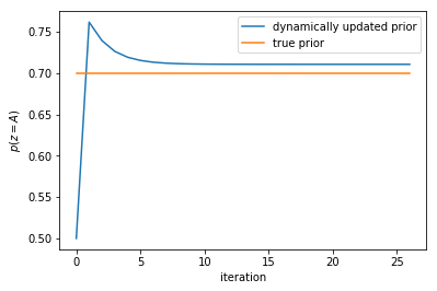
We can see that the prior gradually approachs the true prior as we expected. However, we also notice that there always exists some gap. This might be analytically explained. I will try to think about this in the future.

Conclusion

EM algorithm does work on this example.
To better estimate the parameters, it’s advisable to dynamically update the prior distribution of the hidden variables.

An Introduction to Expectation-Maximization (EM) Algorithm

EM算法详解

Maximum Likelihood Estimation (MLE)

Expectation-Maximization (EM) Algorithm

Apply EM algorithm to practical questions

Implementation and Analysis

The influence of whether dynamically updating the prior or not

Conclusion

CATALOG

FEATURED TAGS

FRIENDS

\(\mathbf{x}^{(1)}\)	01011	\(\mathbf{x}^{(6)}\)	01110
\(\mathbf{x}^{(2)}\)	01111	\(\mathbf{x}^{(7)}\)	01110
\(\mathbf{x}^{(3)}\)	11011	\(\mathbf{x}^{(8)}\)	11011
\(\mathbf{x}^{(4)}\)	00011	\(\mathbf{x}^{(9)}\)	00100
\(\mathbf{x}^{(5)}\)	01010	\(\mathbf{x}^{(10)}\)	01001