In the last post on EM algorithm, we introduced the deduction of the EM algorithm and use it to solve the MLE of the heads probability of two coins. In this post, we will apply EM algorithm to more practical and useful problem, the Gaussian Mixture Model (GMM), and discuss about using GMM for clustering.
First, let’s recall the EM algorithm:
Suppose that we have the observations \(\{\mathbf{x}^{(i)}\}, i=1,\dots,n\). \(\mathbf{x}^{(i)}\) is related with a hidden variable \(\mathbf{z}\) which is unknown to us. The task is to find the MLE of \(\theta\):
$$ \theta_\text{MLE} = \arg \max_{\theta} \sum_{i=1}^{n}\log \sum_{\mathbf{z}} p_\theta(\mathbf{z}, \mathbf{x}^{(i)}) $$ The EM algorithm works as follows:
- Randomly initialize \(\theta\), set the \(\mathbf{z}\) prior \(p(\mathbf{z})\)
- Repeat:
At the \(l^\text{th}\) iteration:
- E step:
set \(Q_{l}^{(i)}(\mathbf{z})=p_{\theta_{l-1}}(\mathbf{z}\vert \mathbf{x}_ i)\) for \(i=1,\dots,n\)- M step:
update \(\theta_{l}=\arg \max_{\theta} \sum_{i=1}^{n}Q_{l}^{(i)}(\mathbf{z})\log \frac{p_{\theta_{l-1}}(\mathbf{z}, \mathbf{x}^{(i)})}{Q_{l}^{(i)}(\mathbf{z})}\)- Update the prior \(p(\mathbf{z})\) (optional)
Until \(\theta\) converges.
Based on the experience on solving coin tossing problem using EM, we can further deform the EM algorithm:
- In the E step, according to Bayes Theorem, we have \(Q_{l}^{(i)}(\mathbf{z})=p_{\theta_{l-1}}(\mathbf{z}\vert \mathbf{x}^{(i)})=\frac{p_{\theta_{l-1}}(\mathbf{x}^{(i)}\vert \mathbf{z})p(\mathbf{z})}{p_{\theta_{l-1}}(\mathbf{x}^{(i)})}=\frac{ p_{\theta_{l-1}}(\mathbf{x}^{(i)}\vert \mathbf{z})p(\mathbf{z}) }{ \sum_{\mathbf{z}}p_{\theta_{l-1}}(\mathbf{x}^{(i)}\vert \mathbf{z})p(\mathbf{z}) }\).
Here \(p(\mathbf{z})\) is the prior of the latent variable \(\mathbf{z}\). Either we initialize it as fixed distribution, or we dynamically update it over each iteration. If the number of the value of the variable \(\mathbf{z}\) is finite and traversable, we can directly compute the sum \(\sum_{\mathbf{z}}p_{\theta_{l-1}}(\mathbf{x}^{(i)}\vert \mathbf{z})p(\mathbf{z})\), and then compute the posterior \(Q_{l}^{(i)}(\mathbf{z})\). For example, in two coin tossing problem, \(\mathbf{z}\) can only be coin A (1) or coin B (0). - In the M step, the objective function
$$\begin{align} L(\theta_{l-1}, Q_{l}^{(i)} ) &= \sum_{i=1}^{n}\sum_{\mathbf{z}}Q_{l}^{(i)}(\mathbf{z})\log \frac{p_{\theta_{l-1}}(\mathbf{z},\mathbf{x}^{(i)})}{Q_{l}^{(\mathbf{z})}}\\ &= \sum_{i=1}^{n}\sum_{\mathbf{z}}Q_{l}^{(i)}(\mathbf{z})\log \frac{p_{\theta_{l-1}}(\mathbf{x}^{(i)}\vert \mathbf{z})p(\mathbf{z})}{Q_{l}^{(i)}(\mathbf{z})}\\ &= \sum_{i=1}^{n}\sum_{\mathbf{z}}Q_{l}^{(i)}(\mathbf{z})\log p_{\theta_{l-1}}(\mathbf{x}^{(i)}\vert \mathbf{z}) + \sum_{i=1}^{n}\sum_{\mathbf{z}}Q_{l}^{(i)}(\mathbf{z})\log \frac{p(\mathbf{z})}{Q_{l}^{(i)}(\mathbf{z})} \end{align} $$ Since \(Q_{l}^{(i)}\) is computed in the E step, in the M step it is treated as something which is independent of \(\theta\). Moreover, the prior \(p(\mathbf{z})\) is also assumed to be independent of \(\theta\). Therefore, the term \(\sum_{i=1}^{n}\sum_{\mathbf{z}}Q_{l}^{(i)}(\mathbf{z})\log \frac{p(\mathbf{z})}{Q_{l}^{(i)}(\mathbf{z})}\) is irrelevant to \(\theta\), and the equivalent updating rule of \(\theta\) can be written as:$$\theta_{l}= \arg \max_{\theta} \sum_{i=1}^{n}\sum_{\mathbf{z}}Q_{l}^{(i)}(\mathbf{z})\log p_{\theta_{l-1}}(\mathbf{x}^{(i)}\vert \mathbf{z}) $$ - Update the prior \(p(\mathbf{z})\). The initialized prior may not be the real prior, therefore, we need to update the prior during iteration. The choice of \(f(\mathbf{z})\) is also the prior distribution which can maximize the objective function in the M step: \(L(\theta_{l-1}, Q_{l}^{(i)})\). In the expression of \(L(\theta_{l-1}, Q_{l}^{(i)})\), only the term \(\sum_{i=1}^{n}\sum_{\mathbf{z}}Q_{l}^{(i)}(\mathbf{z})\log {p(\mathbf{z})}\) is related with \(p(\mathbf{z})\). Therefore, the update rule of \(p(\mathbf{z})\) is:
$$ \min_{f(\mathbf{z})} -\sum_{i=1}^{n}\sum_{\mathbf{z}} Q_l^{(i)}(\mathbf{z}) \log{p(\mathbf{z}) }\\ \text{s.t.}\ \sum_{\mathbf{z}} p(\mathbf{z}) = 1 $$ The Lagrangian function$$L(p(\mathbf{z}), \lambda)= -\sum_{i=1}^{n}\sum_{\mathbf{z}} Q_l^{(i)}(\mathbf{z}) \log{p(\mathbf{z})} + \lambda( \sum_{\mathbf{z}} p(\mathbf{z}) - 1 ) $$ By solving \(\frac{\partial{L(p(\mathbf{z}),\lambda)}}{\partial{p(\mathbf{z})}}=-\sum_{i=1}^{n}\frac{Q_{l}^{(i)}(\mathbf{z})}{p(\mathbf{z})}+\lambda=0\), we have the primal optimum \(p^{\star}(\mathbf{z})=\frac{\sum_{i=1}^{n}Q_l^{(i)}(\mathbf{z})}{\lambda}\). Substituting it to the Lagrangian function, we have the dual function:$$d(\lambda)=-\sum_{i=1}^{n}\sum_{\mathbf{z}}Q_l^{(i)}(\mathbf{z})\log\frac{\sum_{k=1}^{n}Q_{l}^{(k)}(\mathbf{z})}{\lambda}+\lambda(\sum_{\mathbf{z}}\frac{\sum_{k=1}^{n}Q_{l}^{(k)}(\mathbf{z}) }{\lambda} -1)$$ . Therefore, the dual problem is:$$ \lambda^\star=\arg\max_{\lambda} d(\lambda) $$ $$\frac{\partial{d(\lambda)}}{\partial{\lambda}}=\sum_{i=1}^{n}\sum_{\mathbf{z}}\frac{Q_l^{(i)}(\mathbf{z}) }{\lambda}-1=0$$ So we have the dual optimum \(\lambda^\star=\sum_{i=1}^{n}\sum_{\mathbf{z}}Q_{l}^{(i)}(\mathbf{z}) =\sum_{i=1}^{n}1=n\) Therefore, we get the update rule of \(p(\mathbf{z})\):$$ p^\text{new}(\mathbf{z}) = \frac{1}{n}\sum_{i=1}^{n}Q_{l}^{(i)}(\mathbf{z}),\ k=1,\dots,M $$ This deduction uses the Lagrangian Duality Principle, for detail please see my post An Introduction to Support Vector Machines (SVM): Convex Optimization and Lagrangian Duality Principle
Gaussian Mixture Model (GMM)
As indicated by its name, the GMM is a mixture (actually a linear combination) of multiple Gaussian distributions. The probability density function of a GMM is (\(\mathbf{x}\in R^p\)):
where \(M\) is the number of Gaussian models. \(\phi_j\) is the weight factor of the Gaussian model \(N(\mu_j,\Sigma_j)\). Moreover, we have the constraint: \(\sum_{j=1}^{M} \phi_j =1\).
GMM is very suitable to be used to fit the dataset which contains multiple clusters, and each cluster has circular or elliptical shape. For example, the data distribution shown in the following figure can be modeled by GMM.
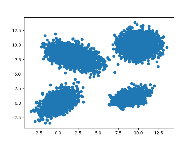 Now the question is: given a dataset with the distribution in the figure above, if we want to use GMM to model it, how to find the MLE of the parameters (\(\phi,\mu,\Sigma\)) of the Gaussian Mixture Model?
The answer is: using EM algorithm!
EM algorithm on GMM parameters estimation
Before we move forward, we need to figure out what the prior \(p(\mathbf{z})\) is for the GMM. Suppose that there are \(M\) Gaussian models in the GMM, our latent variable \(\mathbf{z}\) only has \(M\) different values: \(\{\mathbf{z}^{(j)}=j| j=1,\dots,M\}\). The prior \(p(\mathbf{z}^{(j)})=p(\mathbf{z}=j)\) represents the likelihood that the data belongs to cluster (Gaussian model) \(j\), without any information about the data \(\mathbf{x}\). According to the marginal likelihood we have:
If we compare these two equations with the expression of the GMM, we will find that \(p(\mathbf{z}^{(j)})\) plays the role of \(\phi_j\). In other words, we can treat \(\phi_j\) as the prior and \(p(\mathbf{x}\vert \mathbf{z}^{(j)}; \mu, \Sigma)= N(\mathbf{x};\mu_j, \Sigma_j)\)
Moreover, \(\mathbf{x}^{(i)}\in R^p\). The EM algorithm works as follows:
- Initialization:
We normalize the raw data if necessary, randomly initialize \(\phi, \mu, \Sigma\). - Repeat:
To avoid an overcomplicated expression, we omit the footnote of iteration index \(l\)- E step:
\(\begin{align} Q^{(i)}(\mathbf{z}^{(j)})&=\frac{ p( \mathbf{x}^{(i)}\vert \mathbf{z}^{(j)} ; \mu,\Sigma ) p(\mathbf{z}^{(j)})}{ \sum_{k=1}^{M}p( \mathbf{x}^{(i)}\vert \mathbf{z}^{(k)} ; \mu,\Sigma ) p(\mathbf{z}^{(k)}) } \\ &=\frac{\phi_{j} \frac{1}{(2\pi)^{\frac{p}{2}}\vert \Sigma_j \vert^{\frac{1}{2}} }\exp\{-\frac{1}{2}(\mathbf{x}^{(i)}-\mu_j)^T\Sigma_j^{-1}(\mathbf{x}^{(i)}-\mu_j) \} }{ \sum_{k=1}^{M} \phi_{k} \frac{1}{(2\pi)^{\frac{p}{2}}\vert \Sigma_k \vert^{\frac{1}{2}} }\exp\{-\frac{1}{2}(\mathbf{x}^{(i)}-\mu_k)^T\Sigma_k^{-1}(\mathbf{x}^{(i)}-\mu_k) \} } \end{align}\)
For short we denote \(q_{i,j}=Q^{(i)}(\mathbf{z}^{(j)})\) - M step:
The objective function is:
\(L= \sum_{i=1}^{n}\sum_{j=1}^{M} q_{i,j} \log \phi_{j} \frac{1}{(2\pi)^{\frac{p}{2}}\vert\Sigma_j\vert^{\frac{1}{2}} } \exp\{-\frac{1}{2}{(\mathbf{x}^{(i)}-\mu_j)^T \Sigma_j^{-1} (\mathbf{x}^{(i)}-\mu_j)}\}\)
Update \(\mu\)
We compute the partial derivative:$$\begin{align} \frac{\partial{L}}{\partial{\mu_k}}&=\frac{\partial}{\partial{\mu_k}}\Big[\sum_{i=1}^{n}-\frac{1}{2}q_{i,k}(\mathbf{x}^{(i)}-\mu_k)^T\Sigma_k^{-1}(\mathbf{x}^{(i)}-\mu_k)\Big]\\ &= -\sum_{i=1}^{n}q_{i,k}\Sigma_k^{-1}(\mu_k - \mathbf{x}^{(i)})\\ &= -\Sigma_k^{-1}( \sum_{i=1}^{n}q_{i,k}\mu_k -\sum_{i=1}^{n}q_{i,k}\mathbf{x}^{(i)} )\\ &=0 \end{align}$$ Since \(\Sigma_k>0\), the solution to the above equation is:$$\mu_k^\text{new} = \frac{ \sum_{i=1}^{n}q_{i,k}\mathbf{x}^{(i)} }{ \sum_{i=1}^{n}q_{i,k} },\ k=1,\dots,M$$ Update \(\Sigma\)
let \(\Lambda_k=\Sigma_k^{-1}\), then the objective function is \(L= \sum_{i=1}^{n}\sum_{j=1}^{M} q_{i,j} \log \phi_{j} \frac{\vert\Lambda_j\vert^{\frac{1}{2}}}{(2\pi)^{\frac{p}{2}} } \exp\{-\frac{1}{2}{(\mathbf{x}^{(i)}-\mu_j)^T \Lambda_j (\mathbf{x}^{(i)}-\mu_j)}\}\)
we compute the optimal \(\Lambda^\star_k\) by solving the equation:$$\begin{align}\frac{\partial{L}}{\partial{\Lambda_k}}&=\frac{\partial}{\partial{\Lambda_k}}\Big\{ \sum_{i=1}^{n} q_{i,k}\Big[\frac{1}{2}\log \vert\Lambda_k\vert - \frac{1}{2}(\mathbf{x}^{(i)}-\mu_k)^T\Lambda_k(\mathbf{x}^{(i)}-\mu_k)\Big] \Big\} \\ &=\frac{\partial}{\partial{\Lambda_k}}\Big\{ \sum_{i=1}^{n} q_{i,k}\Big[\frac{1}{2}\log \vert\Lambda_k\vert - \frac{1}{2}\text{tr}\left((\mathbf{x}^{(i)}-\mu_k)^T\Lambda_k(\mathbf{x}^{(i)}-\mu_k)\right) \Big] \Big\} \\ &= \frac{1}{2}\sum_{i=1}^{n} q_{i,k} \Lambda_k^{-1} - \frac{1}{2} \frac{\partial}{\partial{\Lambda_k}} \text{tr}\left(\Lambda_k\sum_{i=1}^{n}q_{i,k}(\mathbf{x}^{(i)}-\mu_k)(\mathbf{x}^{(i)}-\mu_k)^T\right) \\ &= \frac{1}{2}\sum_{i=1}^{n} q_{i,k} \Sigma_k - \frac{1}{2} \sum_{i=1}^{n}q_{i,k}(\mathbf{x}^{(i)}-\mu_k)(\mathbf{x}^{(i)}-\mu_k)^T \\ &=0\end{align}$$ So we have the update rule of \(\Sigma_k\):$$ \Sigma_k^\text{new} = \frac{ \sum_{i=1}^{n}q_{i,k}(\mathbf{x}^{(i)}-\mu_k)(\mathbf{x}^{(i)}-\mu_k)^T }{\sum_{i=1}^{n} q_{i,k} } $$ - update the prior \(\phi_j=\frac{1}{n}\sum_{i=1}^{n}Q^{(i)}(\mathbf{z}^{(j)})\)
- E step:
\(\ \ \ \ \\) Until all the parameters converges.
GMM for Clustering
Suppose that we have use the EM algorithm to find the estimation of the model parameters, what does the posterior \(p_\theta(\mathbf{z}^{(j)}\vert \mathbf{x})\) represent? It actually represents the likelihood that the data \(\mathbf{x}\) belongs to the Gaussian model index \(j\) (or Cluster \(j\)). Therefore, we can use the posterior expression given in the E step above, to the compute the posterior \(p_\theta(\mathbf{z}^{(j)}\vert \mathbf{x}),\ j=1,\dots,M\), and determine the cluster index with largest posterior \(c_x=\arg \max_{j} p_\theta(\mathbf{z}^{(j)}\vert \mathbf{x})\)
Demo
We implement the EM & GMM using python, and test it on 2d dataset.
1
2
3
import numpy as np
import matplotlib.pyplot as plt
from keras.datasets import mnist
1
Using TensorFlow backend.
1
2
3
4
5
6
7
8
9
10
11
12
13
14
15
16
17
18
19
20
21
22
23
24
25
26
27
28
29
30
31
32
33
34
35
36
37
38
39
40
41
42
43
44
45
46
47
48
49
50
51
52
53
54
55
56
57
58
59
60
61
62
63
64
65
66
67
68
69
70
71
72
73
74
75
76
77
78
79
80
81
82
83
def load_data(  num_samples, prior_z_list , mu_list , sigma_list ):
	X=[]
	choice_of_gaussian_model = np.random.choice(len( prior_z_list), num_samples, p=prior_z_list  )
	for sample_ind in range(num_samples):
		gaussian_ind = choice_of_gaussian_model[sample_ind]
		x= np.random.multivariate_normal( mu_list[gaussian_ind], sigma_list[gaussian_ind] )
		X.append(x)

	X= np.asarray(X)
	return X

def EM(X, num_clusters, epsilon = 1e-2, update_prior = True, max_iter = 100000 ):
	x_dim = X.shape[1]
	num_samples = X.shape[0]
	## initialization
	mu = np.random.uniform( size=( num_clusters, x_dim ) )
	## initializing sigma as identity matrix can guarantee it's positive definite
	sigma = []
	for _ in range(num_clusters):
		sigma.append( np.eye(x_dim) )
	sigma = np.asarray(sigma)
	phi = np.ones(num_clusters)/ num_clusters

	count = 0

	while True:
		## E step
		# Q is the posterior, with the dimension num_samples x num_clusters
		Q=np.zeros( [num_samples, num_clusters])
		sigma_det =[ (np.linalg.det(sigma[j]))**0.5 for j in range(num_clusters)  ]
		sigma_inverse = [ np.linalg.inv(sigma[j]) for j in range(num_clusters)  ]
		for i in range(num_samples):
			for j in range(num_clusters):
				Q[i,j]= phi[j]/(   sigma_det[j] ) * np.exp( -0.5 * np.matmul( np.matmul((X[i]-mu[j]).T, sigma_inverse[j]), X[i]-mu[j]))
		Q=np.array(Q)
		Q=Q/(np.sum(Q,axis=1,keepdims=True))

		## M step
		# update mu
		mu_new = np.ones([num_clusters, x_dim])
		for j in range(num_clusters):
			mu_new[j] = np.sum (Q[:,j:j+1]*X ,axis=0 )/np.sum(Q[:,j],axis=0)
		# update sigma
		sigma_new = np.zeros_like(sigma)
		for j in range(num_clusters):
			for i in range(num_samples):
				sigma_new[j] += Q[i,j] * np.matmul( (X[i]-mu[j])[:,np.newaxis], (X[i]-mu[j])[:,np.newaxis].T )
			sigma_new[j] = sigma_new[j]/np.sum(Q[:,j])
		# update phi
		if update_prior:
			phi_new = np.mean( Q, axis=0 )
		else:
			phi_new = phi

		delta_change = np.mean(np.abs(phi-phi_new)) + np.mean( np.abs( mu- mu_new ) )+np.mean( np.abs( sigma- sigma_new ) )
		print("parameter changes: ",delta_change)

		if delta_change < epsilon:
			break

		count +=1
		if count >= max_iter:
			break

		phi=phi_new
		mu= mu_new
		sigma = sigma_new

	## a function used for performing clustering
	def cluster( X ):
		Q=np.zeros( [X.shape[0], num_clusters])
		sigma_det =[ (np.linalg.det(sigma[j]))**0.5 for j in range(num_clusters)  ]
		sigma_inverse = [ np.linalg.inv(sigma[j]) for j in range(num_clusters)  ]
		for i in range(X.shape[0]):
			for j in range(num_clusters):
				Q[i,j]= phi[j]/(  sigma_det[j] ) * np.exp( -0.5 * np.matmul( np.matmul((X[i]-mu[j]).T, sigma_inverse[j]), X[i]-mu[j]))
		Q=np.array(Q)
		Q=Q/(np.sum(Q,axis=1,keepdims=True))
		cluster_info = np.argmax( Q, axis=1)
		return cluster_info


	return {"mu":mu, "sigma":sigma, "phi":phi, "cluster": cluster}
GMM on 2d data points with convex shapes
First let load a small data points
1
2
3
4
real_phi =  [0.2,0.6,0.1,0.1]
real_mu = [ [0,0],[2,8],[10,10],[9,1] ]
real_sigma = [ [[1,0.5],[0.5,1]], [[2,-0.6],[-0.6,1]], [[1,0],[0,1]],[[1,0.3],[0.3,0.5]] ]
X=load_data(10000, real_phi, real_mu, real_sigma )
1
2
for i in range(len(real_phi)):
    print("real phi: ", real_phi[i], " real mu: ", real_mu[i], " real sigma: ", real_sigma[i])
1
2
3
4
real phi:  0.2  real mu:  [0, 0]  real sigma:  [[1, 0.5], [0.5, 1]]
real phi:  0.6  real mu:  [2, 8]  real sigma:  [[2, -0.6], [-0.6, 1]]
real phi:  0.1  real mu:  [10, 10]  real sigma:  [[1, 0], [0, 1]]
real phi:  0.1  real mu:  [9, 1]  real sigma:  [[1, 0.3], [0.3, 0.5]]
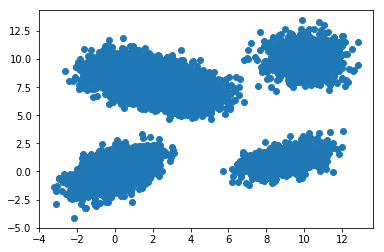
Let’s plot the data and have a look at it.
1
2
plt.scatter( X[:,0], X[:,1] )
plt.show()
Then we apply the EM algorithm, to get the MLE of GMM parameters and get the cluster function
1
2
3
4
5
params=EM(X, num_clusters=4, epsilon= 1E-4)
mu= params["mu"]
sigma = params["sigma"]
phi=params["phi"]
cluster = params["cluster"]
1
2
3
4
5
6
7
8
9
10
11
12
13
14
15
16
17
18
19
20
21
22
23
24
25
26
27
28
29
parameter changes:  28.449669073154364
parameter changes:  17.400927300989974
parameter changes:  0.9644888523985635
parameter changes:  1.0995072448163998
parameter changes:  1.3509364912075696
parameter changes:  1.2308294431017273
parameter changes:  1.3794412438676897
parameter changes:  1.4081227407466508
parameter changes:  1.0857571446279906
parameter changes:  0.7155881044307679
parameter changes:  0.411613512938475
parameter changes:  0.12457364032905578
parameter changes:  0.04685136953006225
parameter changes:  0.0540454165259536
parameter changes:  0.06456840164792643
parameter changes:  0.07771391163679765
parameter changes:  0.09436688134288668
parameter changes:  0.11582159431045104
parameter changes:  0.14421201360388664
parameter changes:  0.1834323022021212
parameter changes:  0.24801453948582258
parameter changes:  0.3558084755399498
parameter changes:  0.5349701481676721
parameter changes:  0.7677886989164794
parameter changes:  0.7666771213539978
parameter changes:  0.5043555266074152
parameter changes:  0.11678542980595268
parameter changes:  0.001048169134691374
parameter changes:  1.550958923947094e-06
1
2
3
4
5
esti_mu= (mu*100).astype(np.int32)/100.
esti_sigma= (sigma*100).astype(np.int32)/100.
esti_phi= (phi*100).astype(np.int32)/100.
for i in range(len(esti_phi)):
    print("esti phi:", esti_phi[i], "esti mu:", esti_mu[i].tolist(), "esti sigma:", esti_sigma[i].tolist())
1
2
3
4
esti phi: 0.09 esti mu: [8.99, 0.99] esti sigma: [[1.07, 0.31], [0.31, 0.51]]
esti phi: 0.19 esti mu: [0.01, 0.01] esti sigma: [[1.0, 0.48], [0.48, 1.01]]
esti phi: 0.1 esti mu: [10.02, 10.02] esti sigma: [[0.92, -0.01], [-0.01, 1.03]]
esti phi: 0.6 esti mu: [2.01, 7.98] esti sigma: [[2.0, -0.61], [-0.61, 1.02]]
If we compare the estimated parameters with the real paramets, we can see the estimation error is within 0.05, and the correspondence between the phi, mu and sigma is also correct. Therefore the EM algorithm does work!
We can perform clustering using the trained cluster model and plot the clustering results
1
2
3
4
5
6
cluster_X = cluster(X)
cluster_index = np.unique(cluster_X)
for ind in cluster_index:
	plt.scatter( X[cluster_X==ind][:,0], X[cluster_X==ind][:,1], color = np.random.uniform(size=3) )
plt.legend(cluster_index)
plt.show()
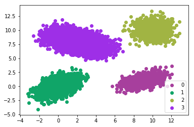
Well, the clustering results are pretty accurate and reasonable! So we can use GMM for unsupervised clustering!
Discussion: As shown the in the figure above, each cluster is actually a convex set.
A convex set $S$ means for any two points $\mathbf{x}1\in S, \mathbf{x}_2\in S$, the linear interpolation $\mathbf{x}\text{int}= \lambda * \mathbf{x}_1 + (1-\lambda)\mathbf{x}_2, 0\leq\lambda\leq 1$ also belongs to $S$
This is pretty reasonable, since Gaussian distribution naturally has a convex shape. However, what the performance of GMM clustering will be for non-convex dataset?
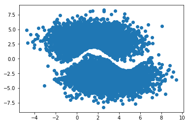
GMM on 2d data points with non-convex shapes
First of all, let prepare the data:
1
2
3
4
5
6
7
8
9
10
11
12
13
14
15
def load_non_convex_data(num_samples=10000, prior_z_list=[0.5,0.5], mu_list=[[np.pi/2, 3], [np.pi*1, -3]], sigma_list=[[[np.pi,0],[0,2]],[[np.pi,0],[0,2]]]):
    X=[]
    choice_of_model = np.random.choice(len( prior_z_list), num_samples, p=prior_z_list  )
    for ind in choice_of_model:
        while True:
            x= np.random.multivariate_normal( mu_list[ind], sigma_list[ind] )
            if ind==0:
                if x[1]>1.5*np.sin(x[0])+0.5:
                    break
            else:
                if x[1]<1.5*np.sin(x[0])-0.5:
                    break
        X.append(x)
    X= np.array(X)
    return X
1
X= load_non_convex_data()
1
2
plt.scatter(X[:,0],X[:,1] )
plt.show()
Use EM algorithm to estimate the parameters of the GMM model.
1
2
3
4
5
params=EM(X, num_clusters=2, epsilon= 1E-2)
mu= params["mu"]
sigma = params["sigma"]
phi=params["phi"]
cluster = params["cluster"]
1
2
3
4
5
6
7
8
9
parameter changes:  7.344997536220525
parameter changes:  2.769657568563131
parameter changes:  0.6826557990296913
parameter changes:  0.8559206668196735
parameter changes:  0.9985169905722497
parameter changes:  0.6972809861725238
parameter changes:  0.16143972260766515
parameter changes:  0.014376638549487432
parameter changes:  0.002146320352925
Let’s see the clustering results:
1
2
3
4
5
6
cluster_X = cluster(X)
cluster_index = np.unique(cluster_X)
for ind in cluster_index:
	plt.scatter( X[cluster_X==ind][:,0], X[cluster_X==ind][:,1], color = np.random.uniform(size=3) )
plt.legend(cluster_index)
plt.show()
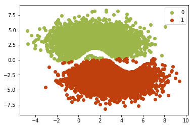
From this figure we can see the real clusters are actually non-convex, since there is a sine-shape gap between two real clusters. However, the GMM clustering resluts always provide convex clutsers. For example, either the blue points set or the red points set is convex. This is determined by the fact that Gaussian distribution has convex shape.
Conclusion
Now we see the ability and shortcoming of the GMM clustering. In the GMM clustering results, each cluster’s region ussually has a convex shape. This actually limits the power of GMM clustering especially on some mainfold data clustring. In the future we will discuss how to cluster such non-convex dataset.
Moreover, this GMM model is not very practical, since for some sparse dataset, when updating the \(\Sigma_j\) in the M step, the covariance matrix \(\frac{ \sum_{i=1}^{n}q_{i,k}(\mathbf{x}^{(i)}-\mu_k)(\mathbf{x}^{(i)}-\mu_k)^T }{\sum_{i=1}^{n} q_{i,k} }\) may not be positive definite (be singular). In this case we cannot directly compute the inverse of \(\Sigma_j\). More works are needed to deal with such cases.
Reference
-
Previous
An Introduction to Expectation-Maximization (EM) Algorithm -
Next
Training a Wasserstein GAN on the free google colab TPU